

CHAPTER 11 | Polys and Subdivs and NURBS, oh my…
17-minute read

Modeling software offers categorically distinct bases for modeling: Polygons (sometimes known as Polys) and NURBS (which, if you’re curious, stands for Non-Uniform Rational B-Splines — a purely algorithmic term you’ll never have to remember). Maya includes a special modification of these called Subdivision Surfaces (or Subdivs for short).
Many paths to (almost) the same goal
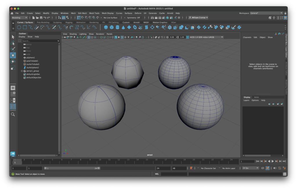
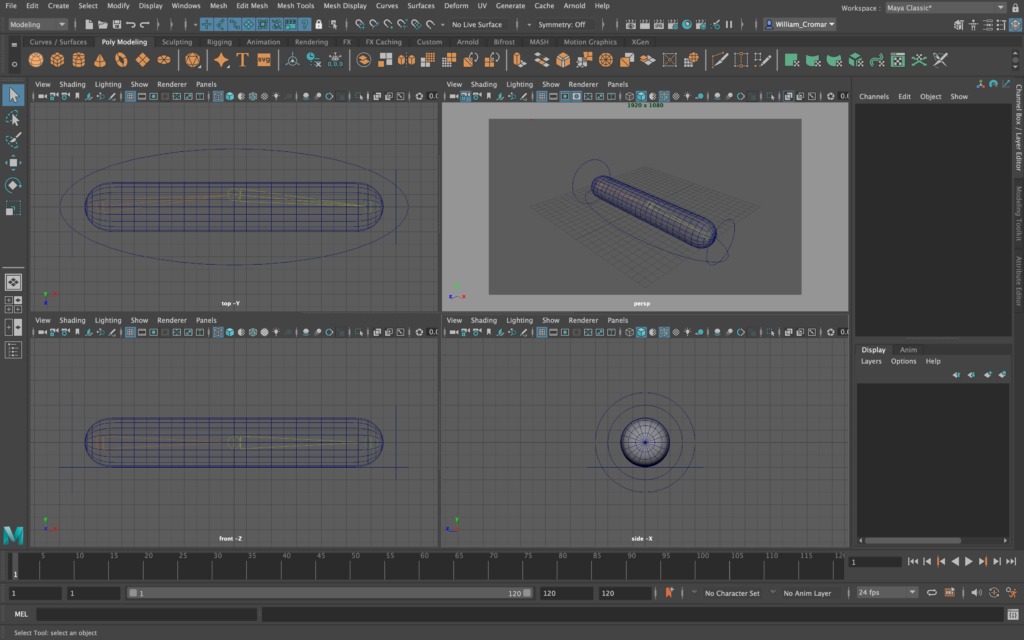
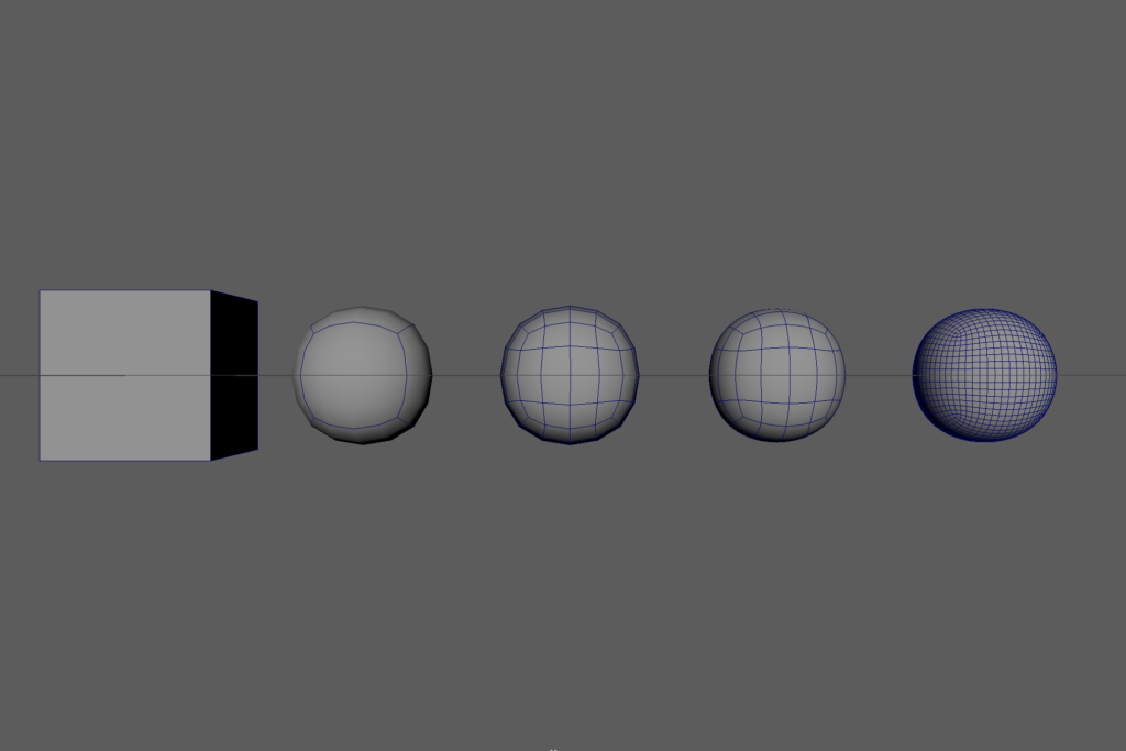
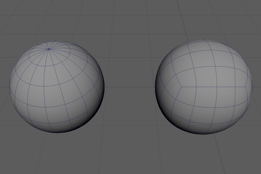
Let’s illustrate an example in Maya that includes that third peculiar option. We open Maya and make four spheres, identical save for their basis, accepting the default values for faces or curves as appropriate. In the figure below, we see a NURBS-based sphere at the left, a Polygon sphere at the right, and Sub-Division models converted from each just behind. When choosing a modeling basis in Maya, NURBS modeling is confusingly found in the Curves/Surfaces modeling tab. In contrast, Polygons are found in their more obviously named adjacent tab. Where do we create Subdivision Surface models? We convert them using the Convert submenu found under Modify in the Menu.
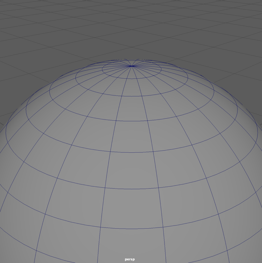
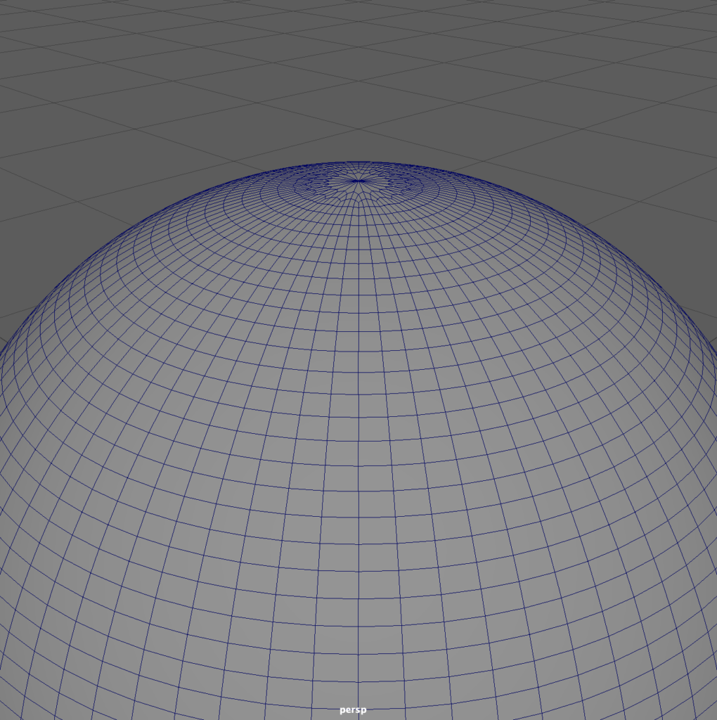
The resulting wireframes all appear radically different, and the Subdiv NURBS sphere doesn’t seem spherical to any rational observer. Now, render the scene and what do you get? Four identical spheres!
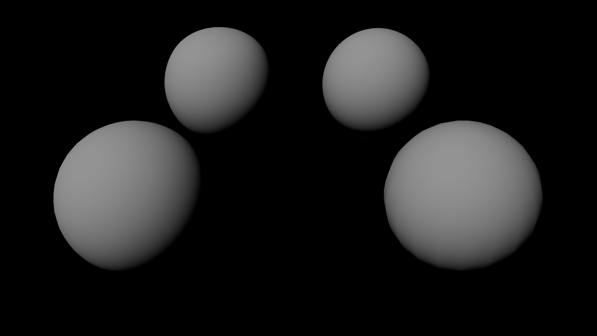
So why do these differences exist if the end product is identical in the render?
The basic differences: a graphic analogy
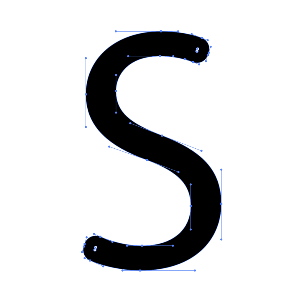
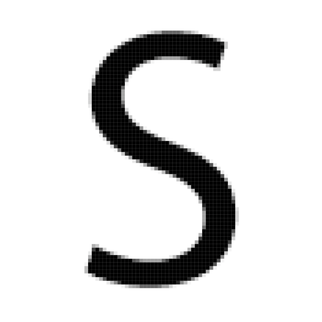
Imagine we’re creating a 2D letter S shape. We have two choices to create it: vector or raster.
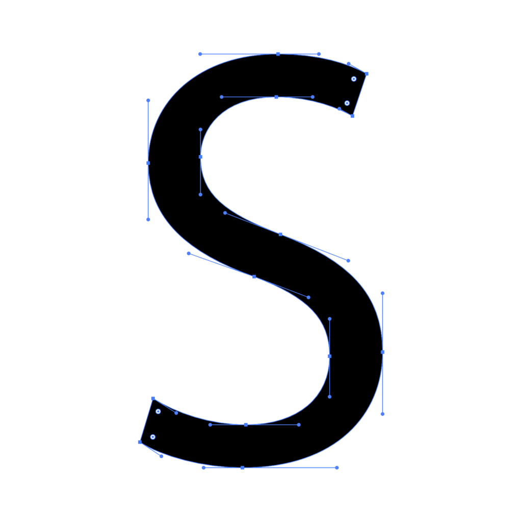
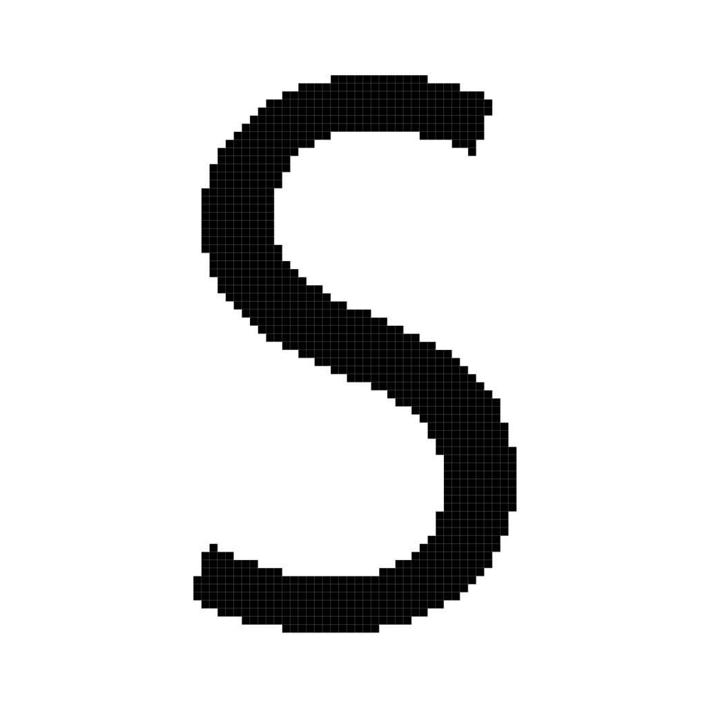
The raster S contains thousands of pixels. The vector S contains dozens of anchors with Bezier handles. The vector shape is scalable, but if we want to place the S in a photograph, the choice is raster.
The difference between NURBS and polygon modeling is similar. Like vector graphics, NURBS modeling creates shape defined by an algorithmic curve. Like raster graphics, polygon modeling creates shape by accumulating a massive number of individual shapes.
Now, say we wish to round corners on the vector S shape. We simply add anchors where we need them. Or, say we might wish to soften the edges in the raster shape. We add shades of gray to create anti-aliasing.
Subdivision surface modeling is analogous to adding curve points or more color pixel data, doing so only where the detail requires it.
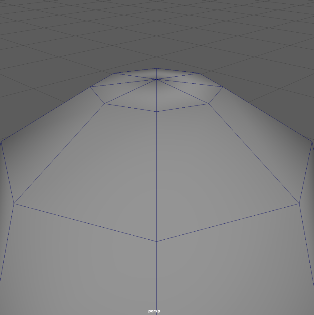
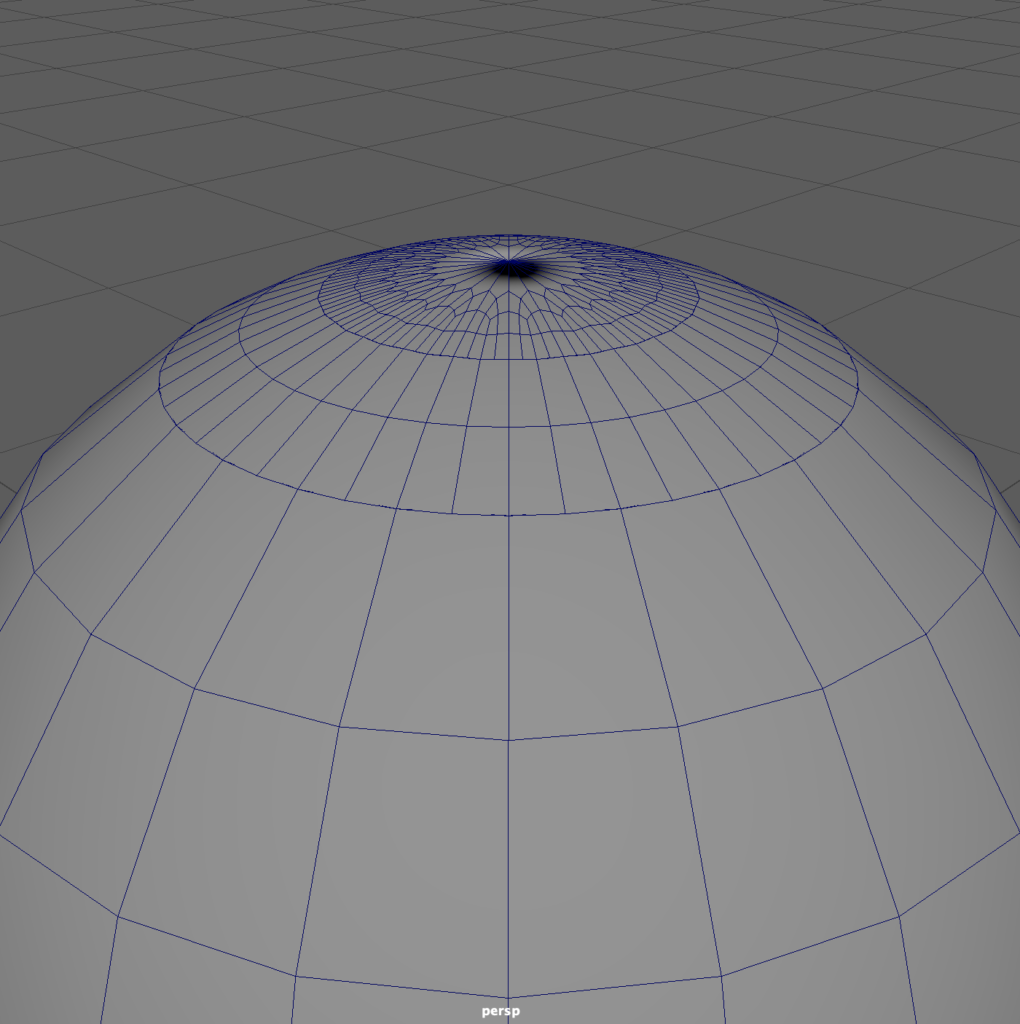
The polygon Subdiv creates more detail at the poles, which seems logical. But notice how the NURBS-based Subdiv appears, because it converts surface control points to polygon vertices!
In Maya, a smooth mesh preview smooths the surface when we hit 3 on the keyboard, but this only works in the viewport; it does not change actual geometry. To make the smooth mesh geometry stick, we use Modify > Convert > Smooth Mesh Preview to Polygon.
From this, we might conclude NURBS is the better choice, but each modeling environment has its pros and cons.
NURBS modeling
Other analogies can help us understand what’s going on under the hood with NURBS. In traditional mechanical drafting, drawing curves for a surface like a boat hull was a tricky problem solved using a flexible physical spline secured by weights. The anchor points on a digital Bezier curve are analogous to the weights that fixed the curved drafting spline.
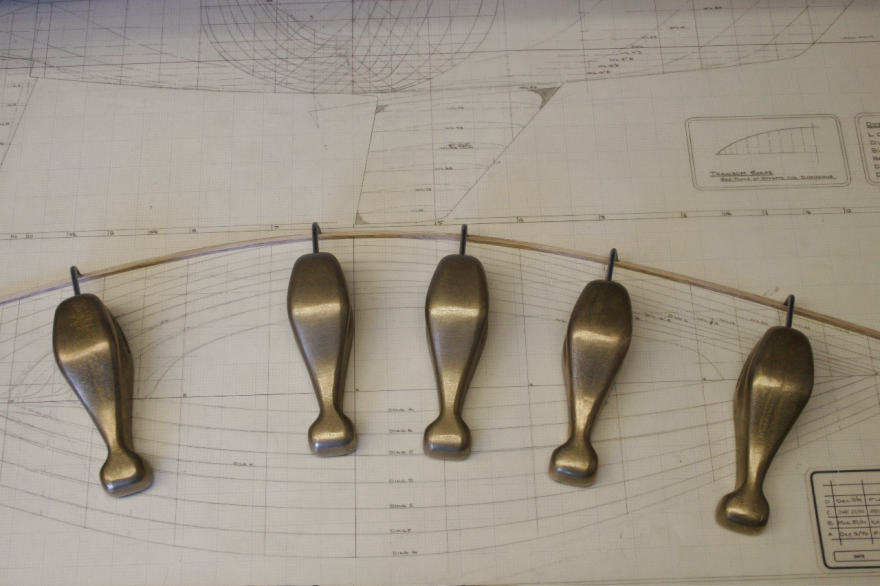
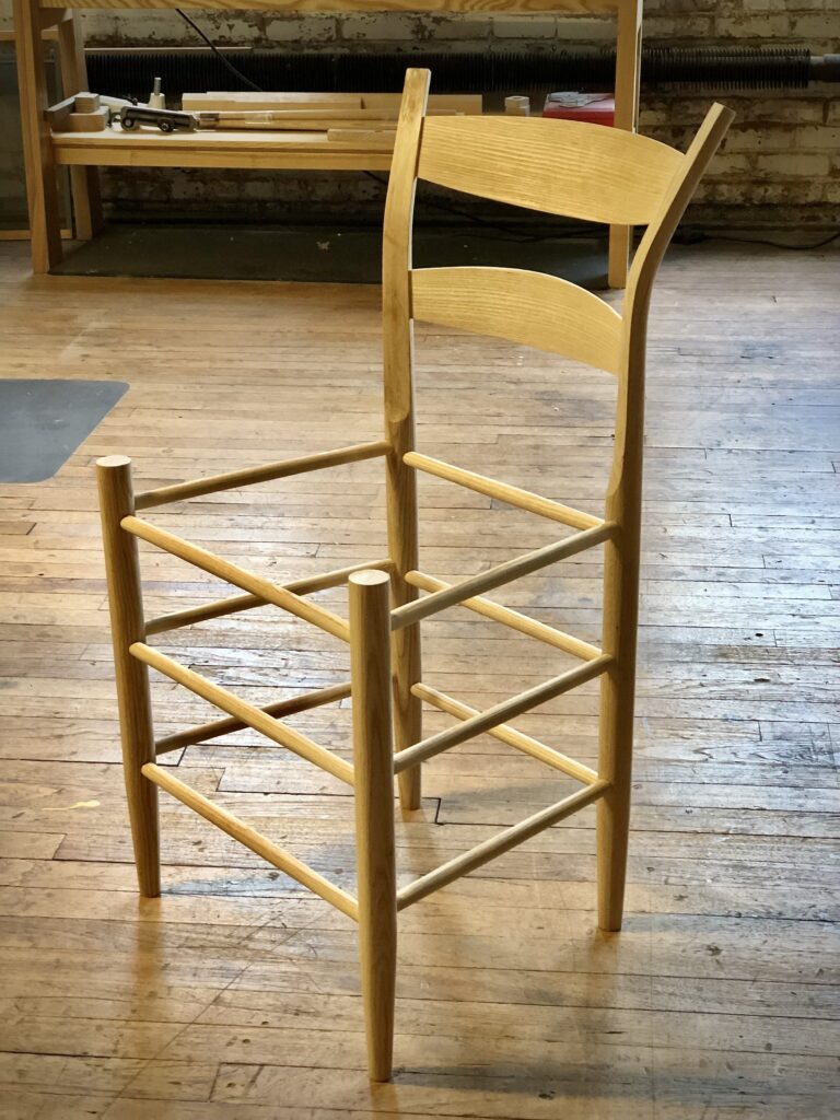
Another analogy is found in the curves created by steam-bending wood for furniture. Wood is held in place with forms and clamps during this process. Clamps are analogous to curve anchor points; forms provide the tension and compression that are analogous to Bezier handles.

These analogies are helpful but limited to bends along a 1D line or a 2D plane. NURBS curves can develop those kinds of bending, but they also occur in a multi-directional 3D context. Another analogy can help us visualize this: containers manufactured by casting plastic inside a mold. Blow molding uses a combination of tension created by pressurized air and compression created by a mold to conform material to a shape. It’s the physical equivalent of a NURBS hull, which we’ll describe below. The hull that develops our NURBS sphere primitive is the 3D equivalent of 2D anchor points and Bezier handles.
Because curves define a surface in a NURBS model, scaling is not a problem. The curves maintain a precise shape regardless of size. The curves are defined by a few control points, so an algorithm recalculates the form when the model is scaled.
Anatomy of a NURBS object
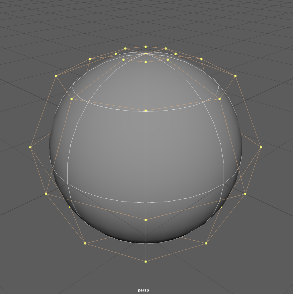
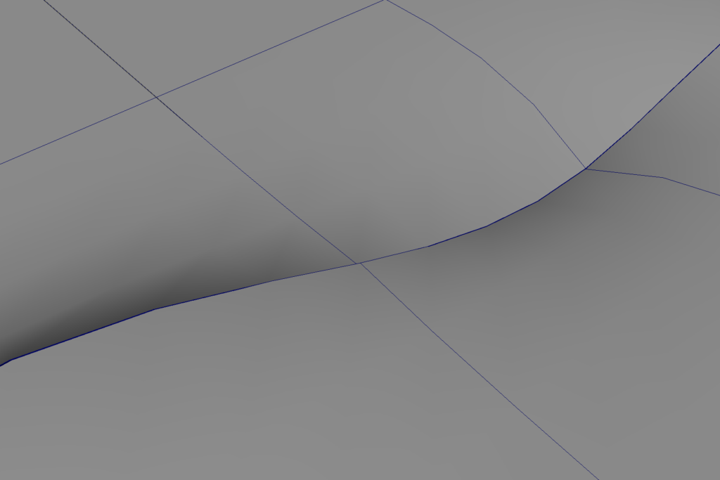
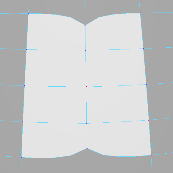
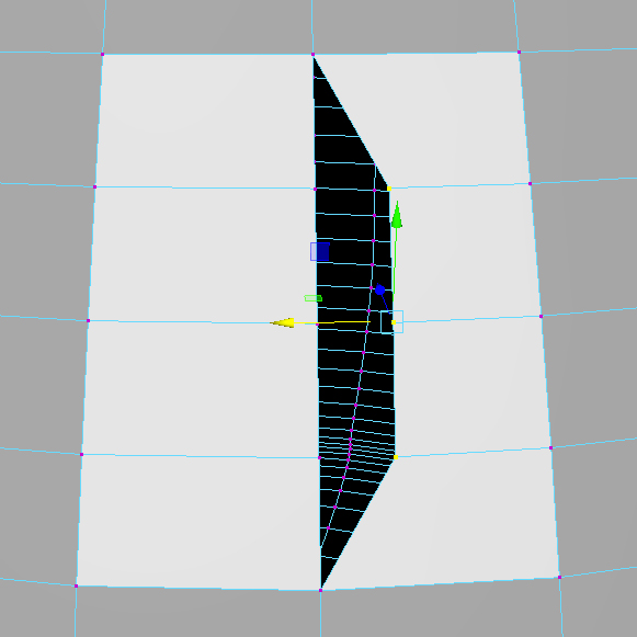
A NURBS surface is defined by some curious elements for those who are familiar with polygon modeling. It’s tempting to think of a Control Point, also known as a Control Vertex or CV, as equivalent to a polygon Vertex (see below), but a CV is often not congruent with the surface since its role is similar to that of a Bezier handle. CVs are grouped into a matrix called a Hull, which connects CVs to visualize the flow of these points as they project onto the NURBS surface. Where these hull lines project, we can see Isoparms, which are tempting to compare to polygon Edges. Where isoparms intersect, they create a Surface Patch, or Patch, which feels like a polygon Face.
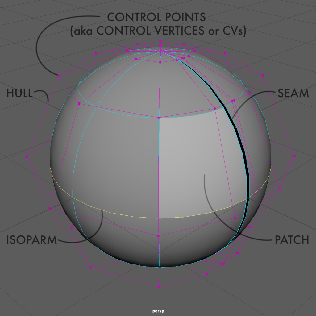
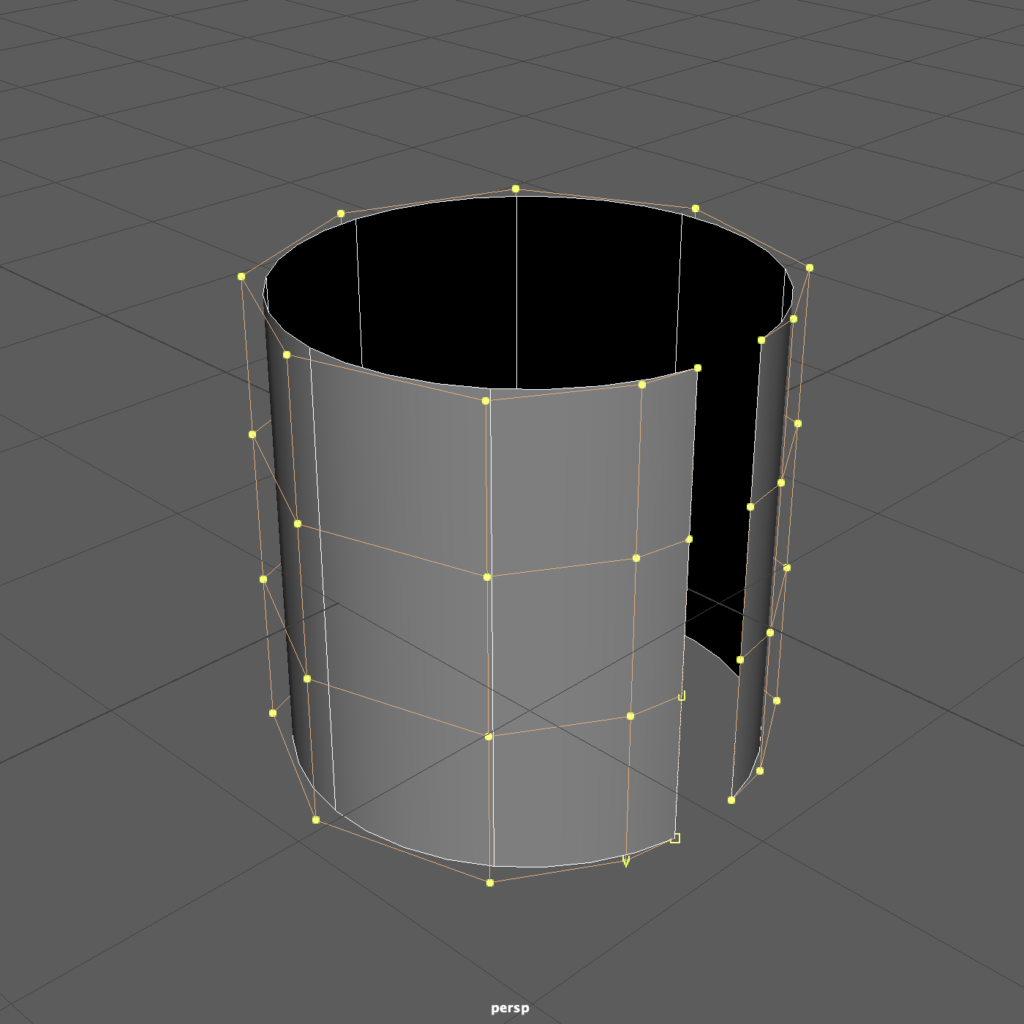
Perhaps the most curious departure from polygon modeling is the ever-present Seam. Every NURBS surface has four edges, which often “stitch” together to create uniform surfaces, not unlike swatches of fabric sewn together at their seams to create a garment. In our illustration, we exaggerate the seam by opening it up a degree or two. But in the sphere, we only see two sides, not four! This is because the poles of the sphere are a special case, where the CVs that control the “north pole” and the “south pole” are congruent. A clearer expression of the four sides of a NURBS surface might be seen in a cylinder with a gap in its sweep.
NURBS pros and cons
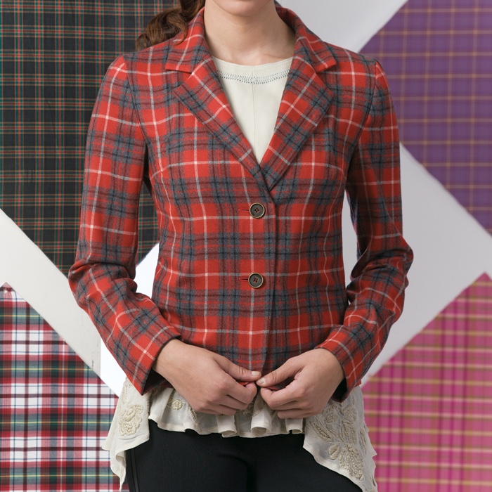
Seams are intimidating! Even experienced modelers must work with care. Creating a NURBS model is analogous to sewing patterned cloth so it fits the contour of the body while matching the pattern. With a carefully planned workflow, we can create a well-crafted garment.
NURBS seams can be painful to correct, but by attaching them, we arrive at a smooth result, though at the cost of curve change. By stitching, we get a crease but maintain the curve. No pun intended, but there’s a steep learning curve associated with these tools.

After we repair this seam, it looks like a single surface. Therefore, difficulties in the NURBS workflow make it a rare choice for graphic applications. However, the precision of NURBS makes it useful for product design.
NURBS modeling has the advantage of overhead efficiency. The amount of information required to create a form in NURBS is significantly smaller, so rendering a NURBS object is comparatively faster. However, NURBS are notoriously difficult to rig or deform! We often find them playing a supporting role in rigging: simple NURBS curve controllers provide an animator with tools in the viewport to move a rig while remaining hidden in the render.
Applying textures to NURBS can be challenging. And though it is a logical choice for design, some fabrication environments may not be compatible with NURBS. We must often convert NURBS to polygons before 3D printing or rendering, resulting in quality loss or increased complexity.
Polygon modeling
A polygon mesh can approximate forms, from simple geometric primitives to complex organic geometry. A mesh can be analogous to a sculptural form made from wire cloth or wire mesh.
In a wireframe view, we can get a sense of the overall form of an object as if it were transparent. If we describe NURBS modeling as being precise, we can say polygon modeling can be accurate.
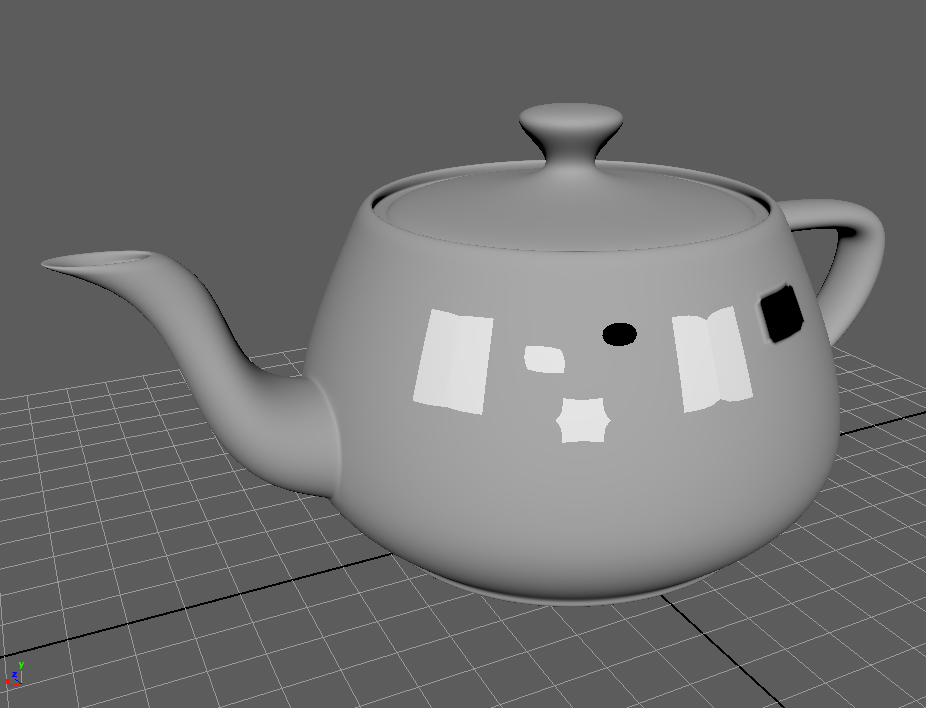
Utah Teapot with a poly-count of approximately 1000 faces
Utah Teapot with a poly-count of approximately 10,000 faces
The accuracy of a polygon model is a function of resolution: the number of polygons being used to describe the surface at a particular size. Above we see two different polygon counts for the same object, the Utah Teapot. This is analogous to the number of pixels present in a raster image: the more data, the more accuracy.

Anatomy of a polygon object
Polygons are straight-sided shapes, defined in 3D coordinate space by points with no dimension, or Vertices. These are comparable to, but not the same as, NURBS CVs. Where a CV is independent of the surface it controls, a polygon vertex is congruent with the object surface.
The 1D lines that connect vertices are called Edges. They are roughly analogous to NURBS Isoparms. The 2D area created by 3 or more vertices connected by edges is called the Face. Faces are somewhat analogous to NURBS surface Patches.
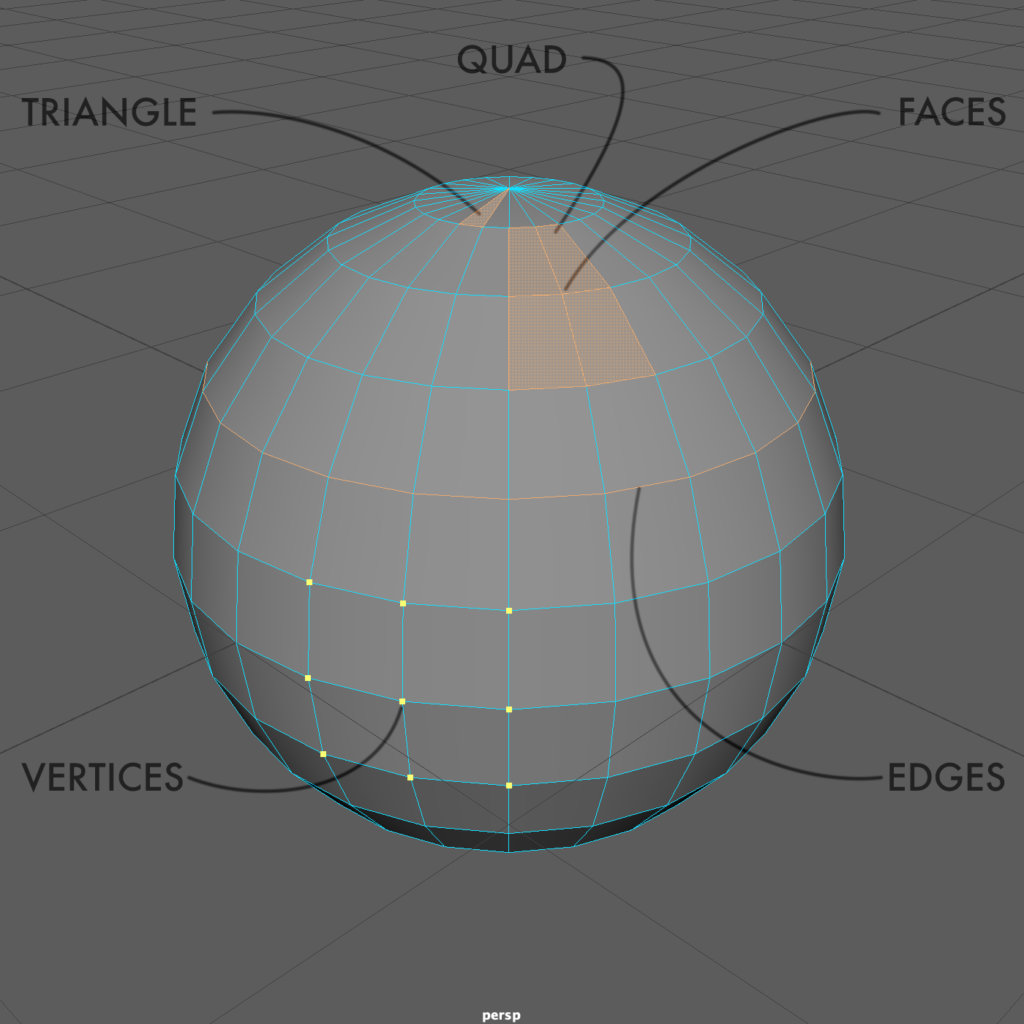
In polygon modeling, we use 3-sided polygons called Triangles or 4-sided polygons called Quads, an abbreviation of the term Quadrilaterals. We generally avoid working with polygons of more than 4 sides, known as N-gons.
When many Faces are connected by sharing Edges and Vertices, this creates a network called a Polygon Mesh. We create 3D polygonal models using polygon meshes.
Polygon pros and cons
Relative to NURBS, polygon models are easy to texture, animate, and deform. They have a natural and intuitively understood UV mapping logic, which means that you can apply textures to them without the hassle we often find with NURBS. They are very compatible with most 3D software, digital fabrication environments, and renderers. While any good model takes careful planning, we can sculpt and edit a polygon model and get real-time intuitive feedback from it.
However, polygon models have some drawbacks. They are less flexible, less precise, and suffer when scaled as compared to NURBS. Polygon surfaces are approximations of curves and surfaces, so they cannot represent any curving surface without introducing distortion. They don’t play well with functions like lofting, revolving, trimming, or blending, so forms that rely on these operations can get quite procedurally additive and overly dependent on combining multiple meshes.
We mentioned earlier Maya’s use of a smooth mesh preview to compensate for the low fidelity of polygon modeling. This creates a large, inefficient dataset, making a high polygon count difficult to store and work with.
Normals to the rescue
So if the polygon count gets so large that a computer can’t process it, how can some relatively low-poly models appear to be so smooth? Normals can provide a way to give the illusion of a smooth surface. They come in two flavors: Face Normals and Vertex Normals.
A Face Normal is an algorithmic vector perpendicular to a polygon face indicating the direction a surface is facing and is often used in graphics for rendering.
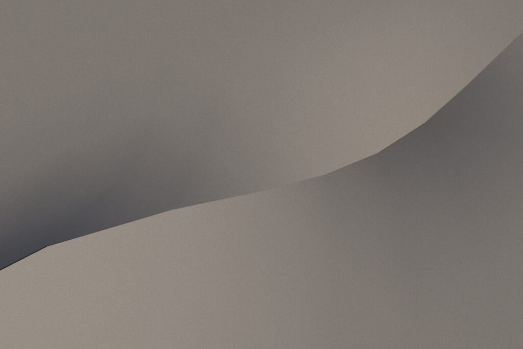
A Vertex Normal’s direction is not intrinsically directional because, unlike a plane, it has no inherent orientation, so it is a property that can be set. A soft edge normal is set to 180 degrees, making any edges disappear. A hard edge normal is set to 0 degrees, making edges appear sharp.


Note in the illustrations that setting a soft edge is not the same thing as creating a smooth mesh preview. The silhouette of the soft edge mesh still feels faceted. We only get the smooth silhouette by combining the smooth edge with soft edge normals. On the other hand, a smooth edge preview can be set with hard edge normals, revealing the additional faces created in the so-called smooth mesh!
Problematic polygons
Rendering and 3D printing both like clean meshes, but operations like Booleans or conversions from NURBS don’t necessarily create the cleanest models.
Many inadvertent problems can arise that can make your mesh a bit wonky if not outright breaking it. We’ve deliberately created several common mesh problems in the Utah Teapot we saw earlier. These include congruent vertices, polygon edge definition, holes, “rips” in the mesh, and reversed normals, all described with their fixes below.
Congruent vertices
Congruent vertices can make a real mess and are tough to spot. Without smoothing they are impossible to detect. Congruent vertices can happen during NURBS conversion, inadvertently when performing point snaps, and careless beveling on a flat surface. To fix, select one of the congruent vertices, move it, and then perform a Target Weld.
Polygon definition
We need to avoid n-gons: any polygon larger than a triangle or a quadrangle. When cleaning a model for printing or rendering, we keep our models consistently defined by triangles or quads. Use Mesh > Triangulate or Quadrangulate as appropriate to the situation. This will solve most problems, but sometimes we need a more granular solution: delete edges or add edges using the Multi-Cut Tool.
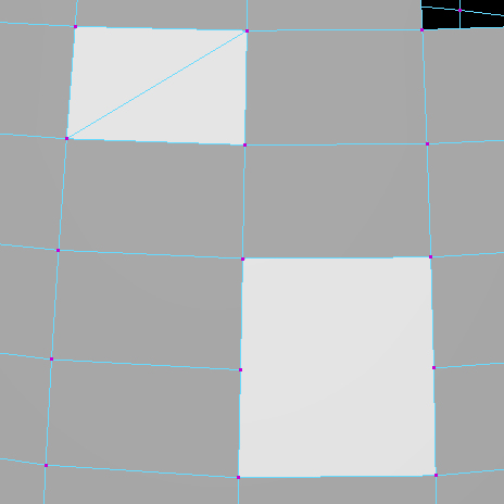
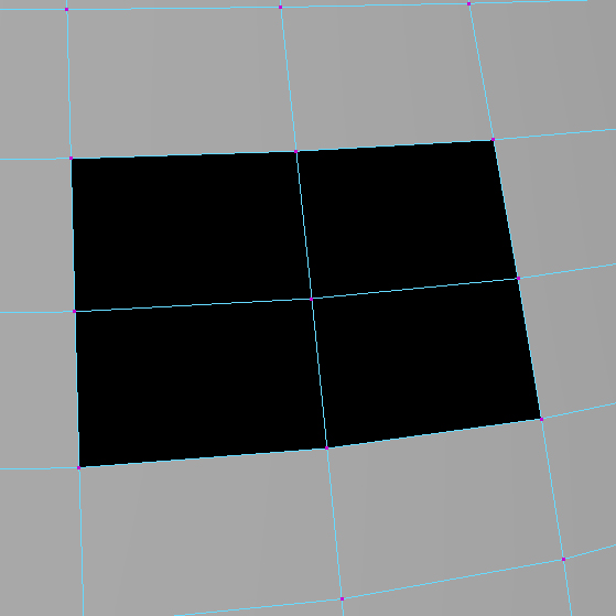
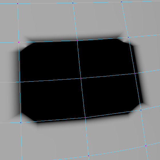
Holes
That dark area is not a different material applied to a face: it’s a missing face altogether. To fill a hole, select the edges of the hole and go to Mesh > Fill Hole.
“Rips”
A “rip” in the mesh is an unholy combination of a hole with congruent vertices. We see these often occur when we perform Boolean operations. They can break an otherwise decent model. The fix is identical to the fix for congruent vertices. Use a vertex move followed by a Target Weld. You can see how, even with smoothing in operation, rips are pretty tricky to spot.
Reversed normals
Because a normal defines the “front” and “back” faces of a polygon, poorly defined normals often won’t even print or render, creating a hole in the output. We must set the normals to face the exterior of the model so that a printer or render engine can “see” the faces. Using Mesh Display > Reverse, open the dialog and check Reverse normals on Selected faces.
Normals can also develop odd angles during modeling; the “front” is sort of facing “sideways.” We can recognize this by seeing funny highlights or shadows that seem out of place on the mesh. Fix these “twisted” normals by going to Mesh Display > Set to Face.
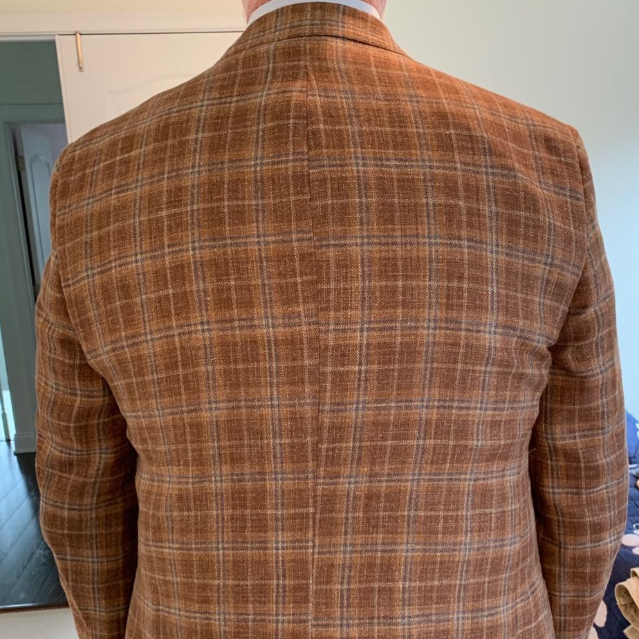
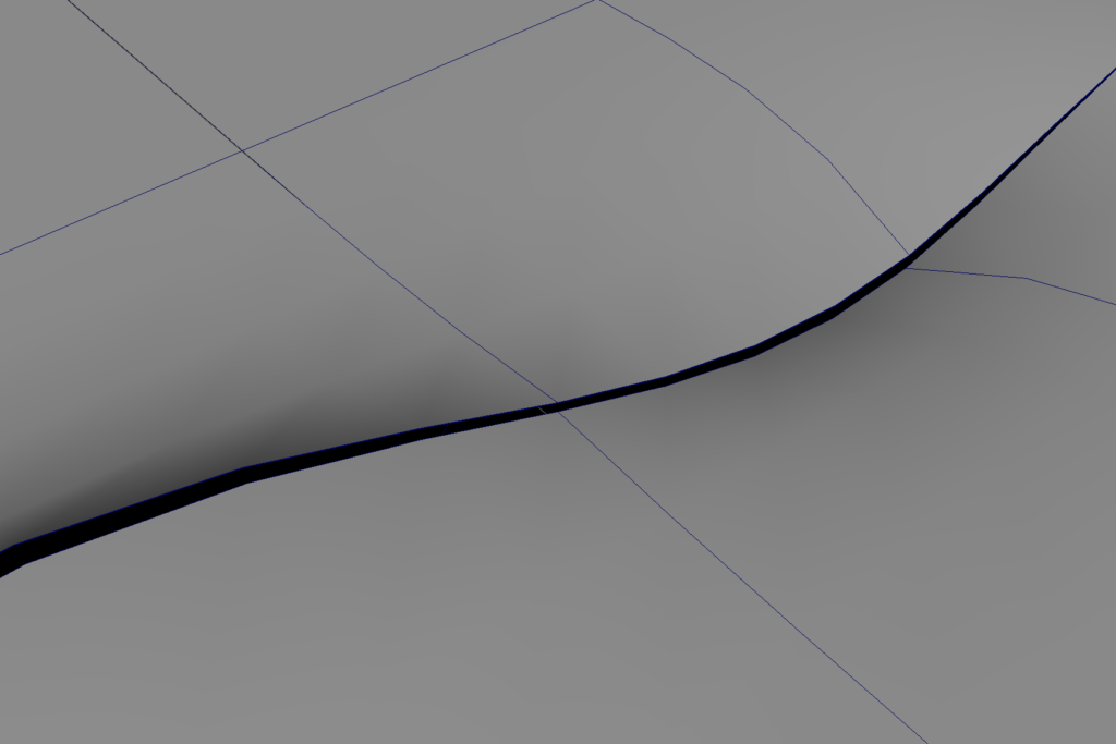
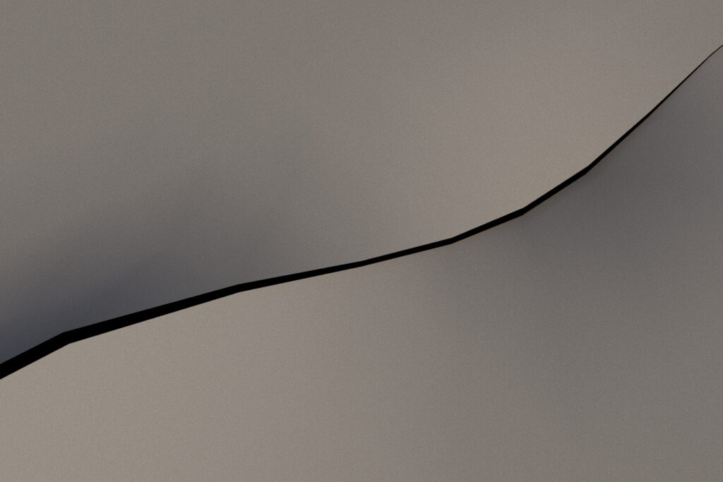
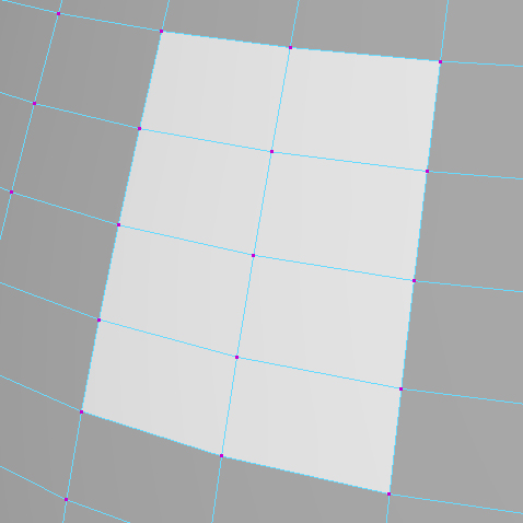
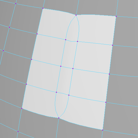
Non-planar faces: not really broken, but…
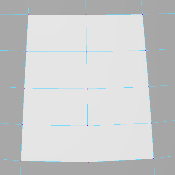
A non-planar face is a polygon whose vertices are not in the same plane. A triangle is always a planar object, but a quad can often inadvertently generate one point that is out of plane with the other three. In practical terms, we may find many quads in a complex model are non-planar, and minor deviations from planarity don’t require a fix. However, it can be desirable to flatten a quad now and then.
To identify a non-planar face can be super tricky. We’ve deliberately not highlighted our non-planar faces here: can you identify them?
If we’re working with Maya, we can visualize hard-to-find non-planar polygons by selecting Display > Polygons > Non-planar Faces, and the software will reveal them for us.
To correct non-planarity we can use the Multi-Cut Tool to split them into triangles or Mesh > Retopologize the faces. A simple fix is to perform a Mesh > Cleanup with the non-planar fix option selected. However, this can lead to some funky issues with the phenomenon known as Edge Flow.
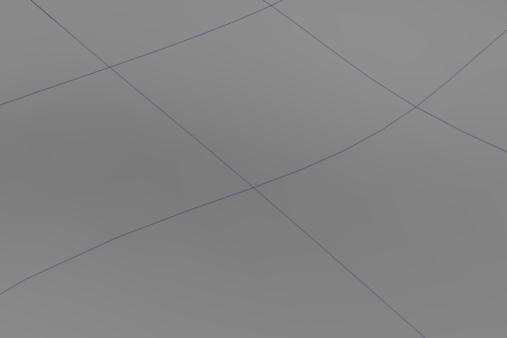
Edge flow
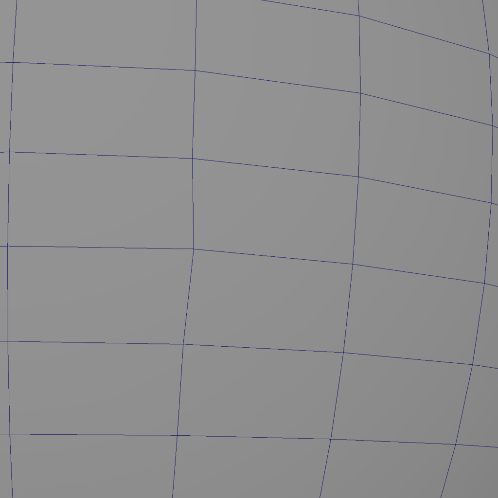
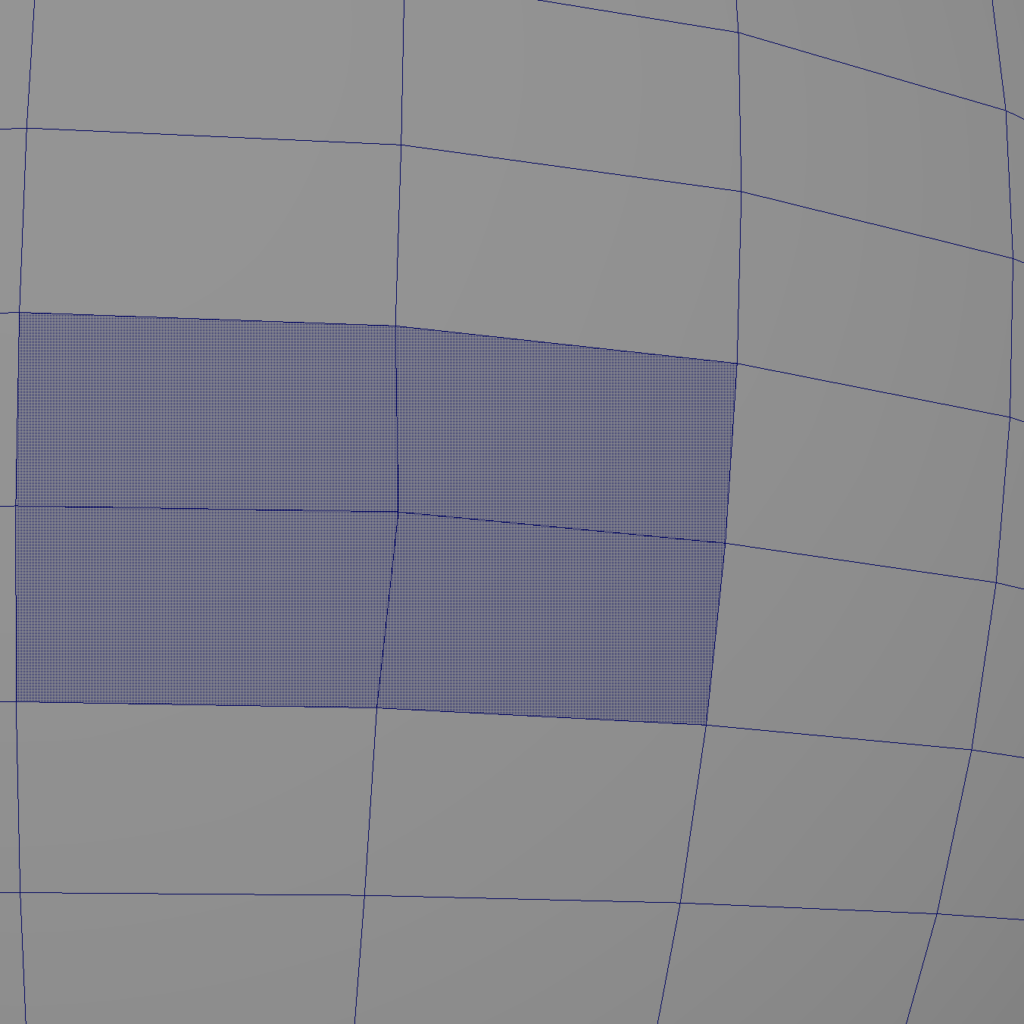
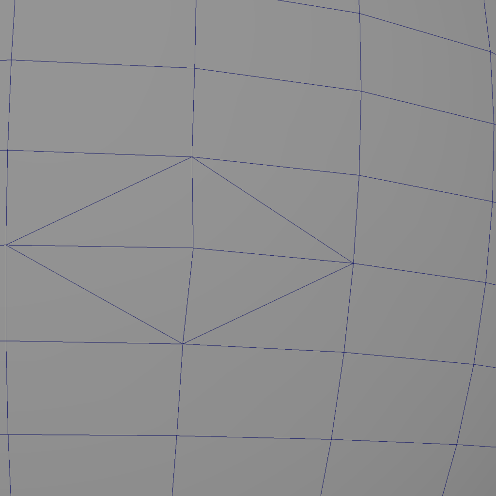
Edges between faces in a polygon mesh are shared. By maintaining a good Edge Flow, we generate models that texture and animate more fluently. As we follow the trajectory of a flow, it should define a clear path through the model. Jagged, disfigured, out-of-scale polygons are all indicators of bad edge flow.
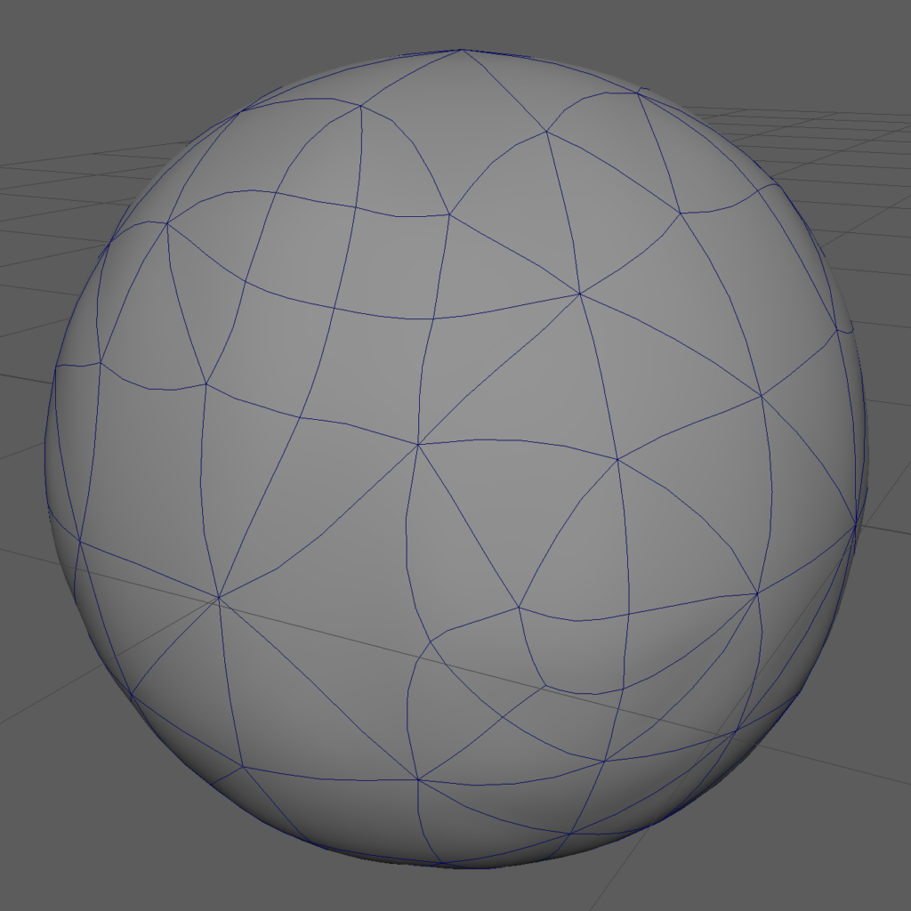
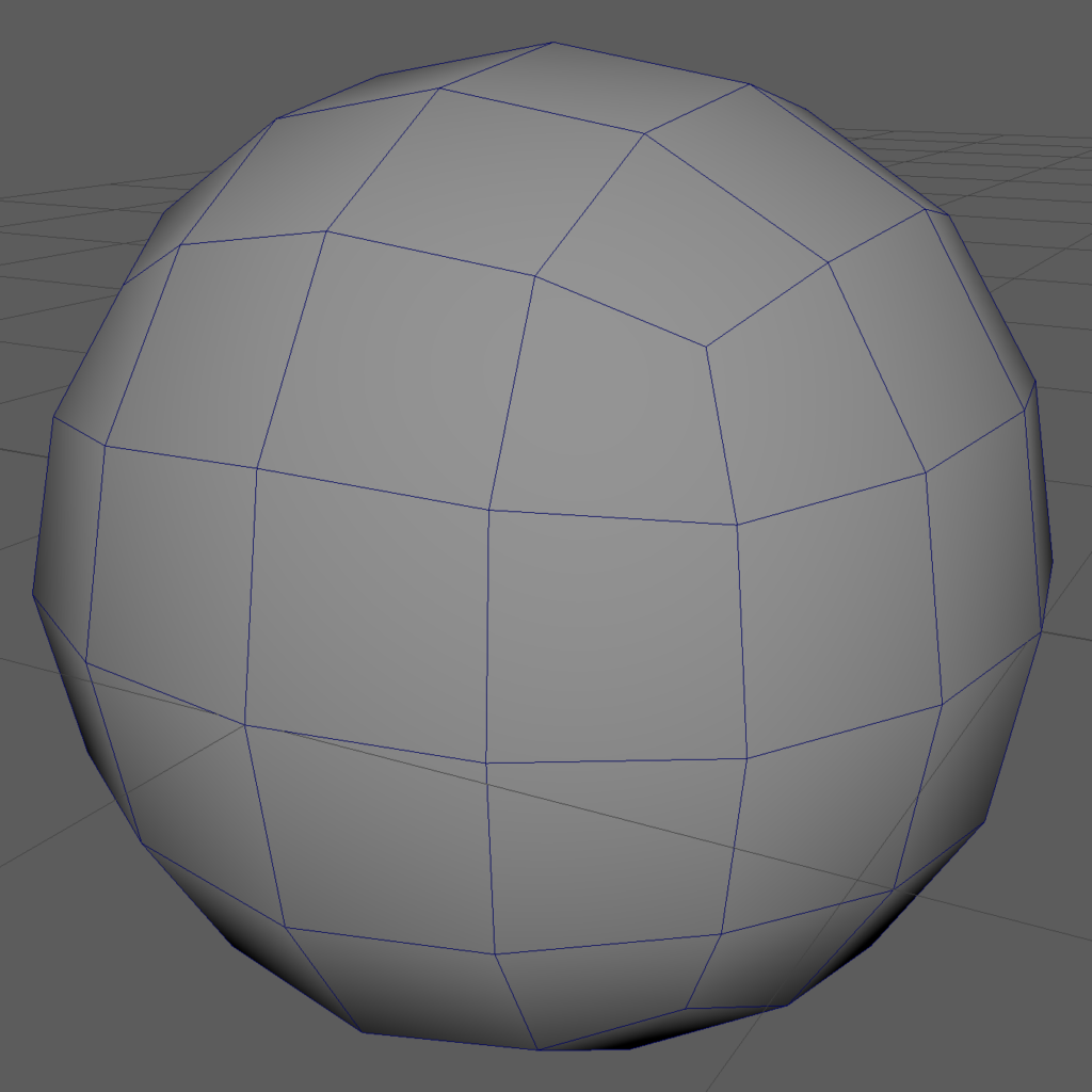
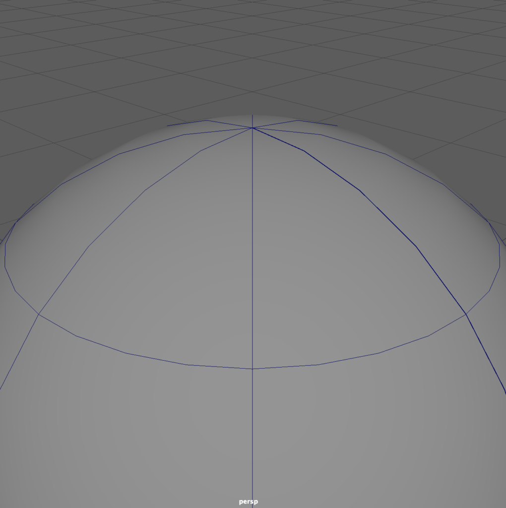
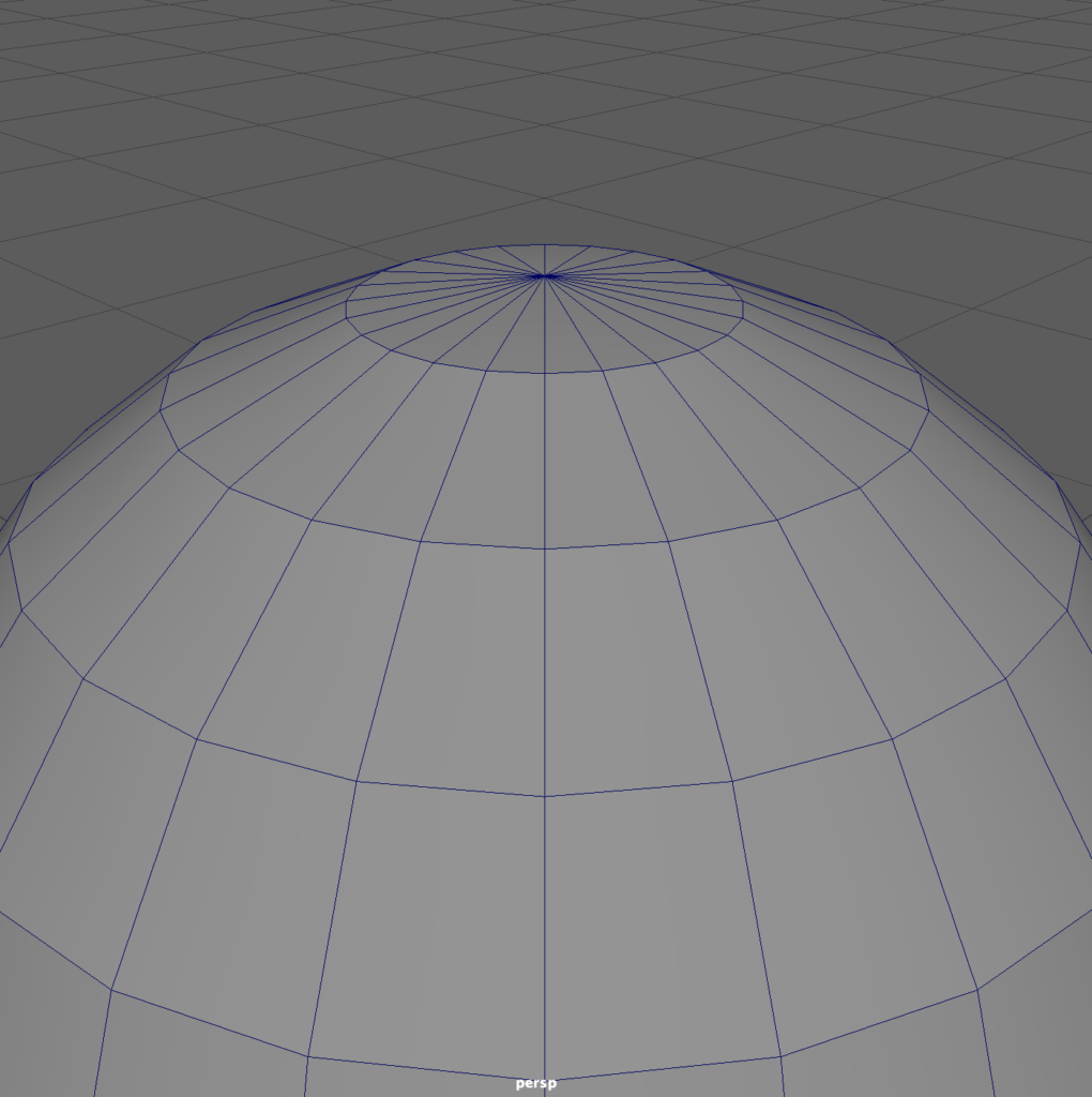
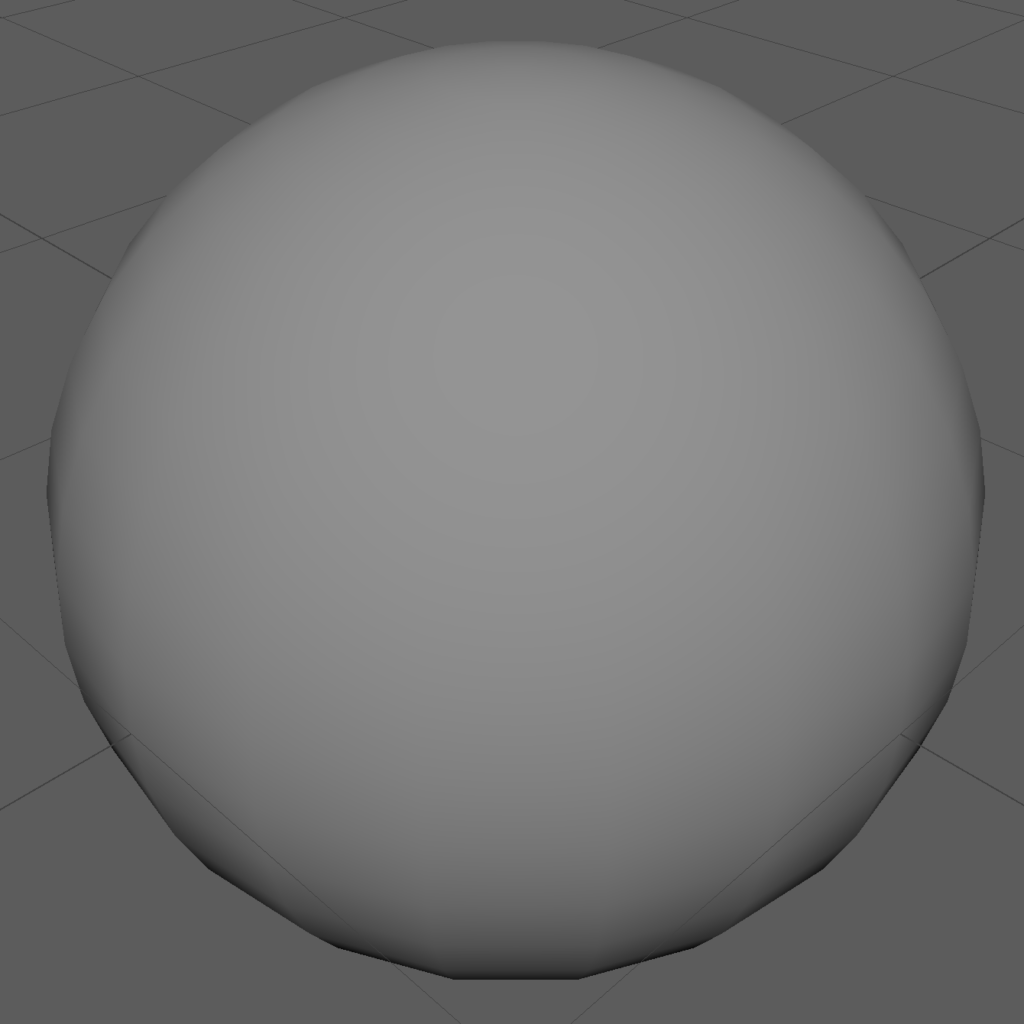
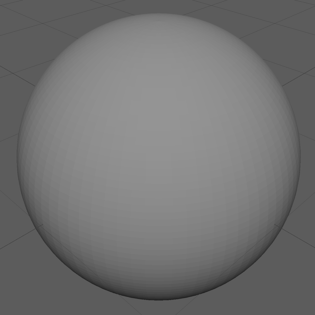
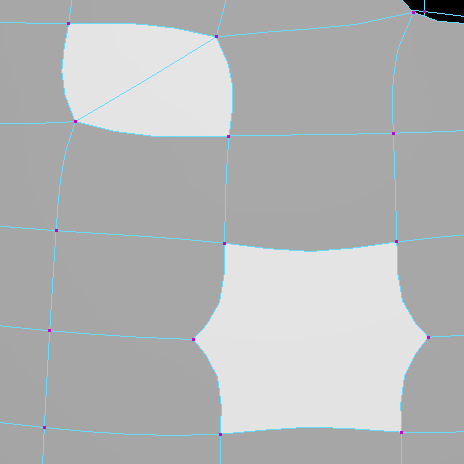
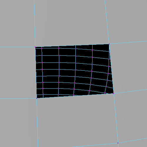
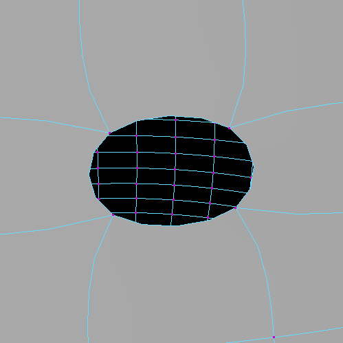
The sphere with bad edge flow is a mix of triangles, quads, and n-gons. It has a uniform surface, so there is no logic to the arrangement of large and small polygons. When looking at the smooth mesh preview, we detect pinching in the surface. By comparison, the sphere with good edge flow is based on uniformly distributed quads of a similar scale. Upon smoothing, we observe no surface distortion.
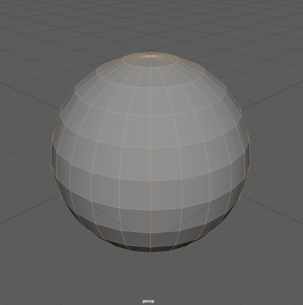
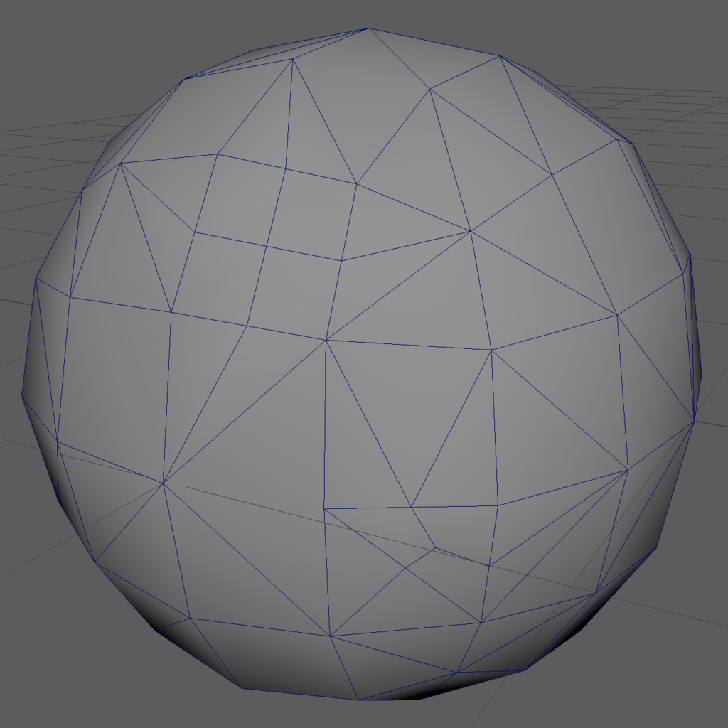
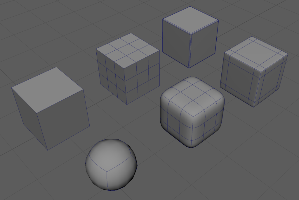
Incidentally, we create that good sphere from a quad ball, which we can find as a primitive solid in some software packages. In Maya, it’s easy to make one in a few steps, starting with a simple cube. Apply a smooth mesh preview to the cube using 3 on the keyboard, then use Modify > Convert > Smooth Mesh Preview to Polygons. Smooth the result again, and convert again, if you want more detail.
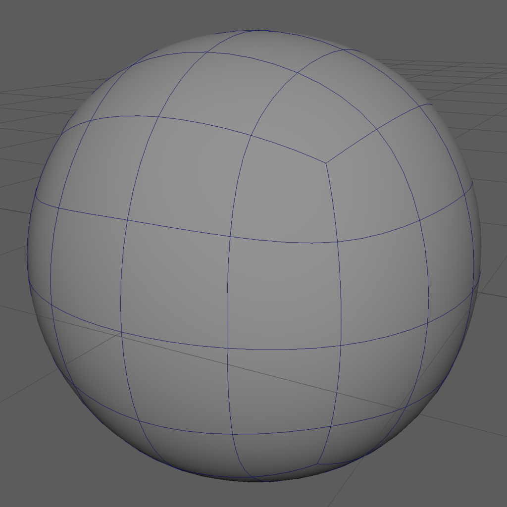
We love the quad ball! Compare it with the standard polar sphere primitive, with its multiple triangles at the poles. While both exhibit good edge flow, the quad ball eliminates the mixture of quads and tris that can often create texturing, distortion, or animation problems. Try modeling a human head from both primitives — the quad ball wins. One big reason why is that quads are superior when using subdivision surfaces for complex detail.
Subdivision surfaces
Creating a polygon mesh by hand can result in a blocky model. To generate every polygon at the size required for smoother detail is impossible, so we turn to subdivisions. If we provide the “outline” of a model in the form of a polygon mesh, the software can subdivide or “smooth” it to create a higher resolution and more detail.
Across all 3D software packages, subdivision generally applies to the principle of dividing a face into more faces where we need more detail. In Maya, we find a type of object called a Subdivision Surface, or Subdiv, which combines features of NURBS and polygons while adding detail where we need it. Instead of uniformly smoothing a mesh of a hand, for example, it will place more detail around a finger joint, and leave the back of the hand with fewer, larger faces.
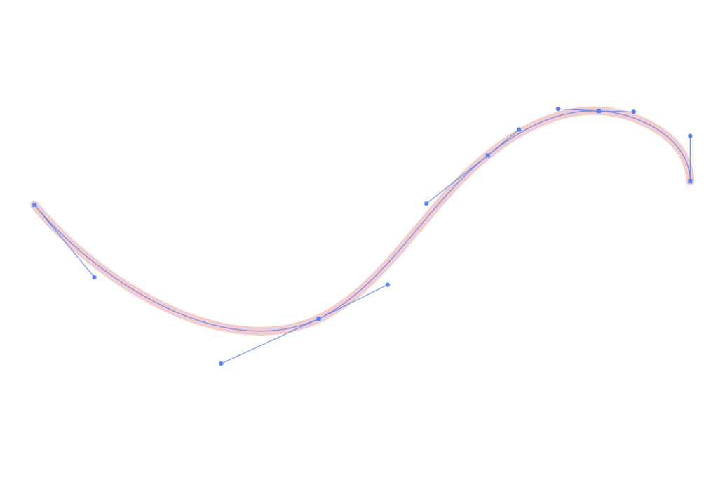
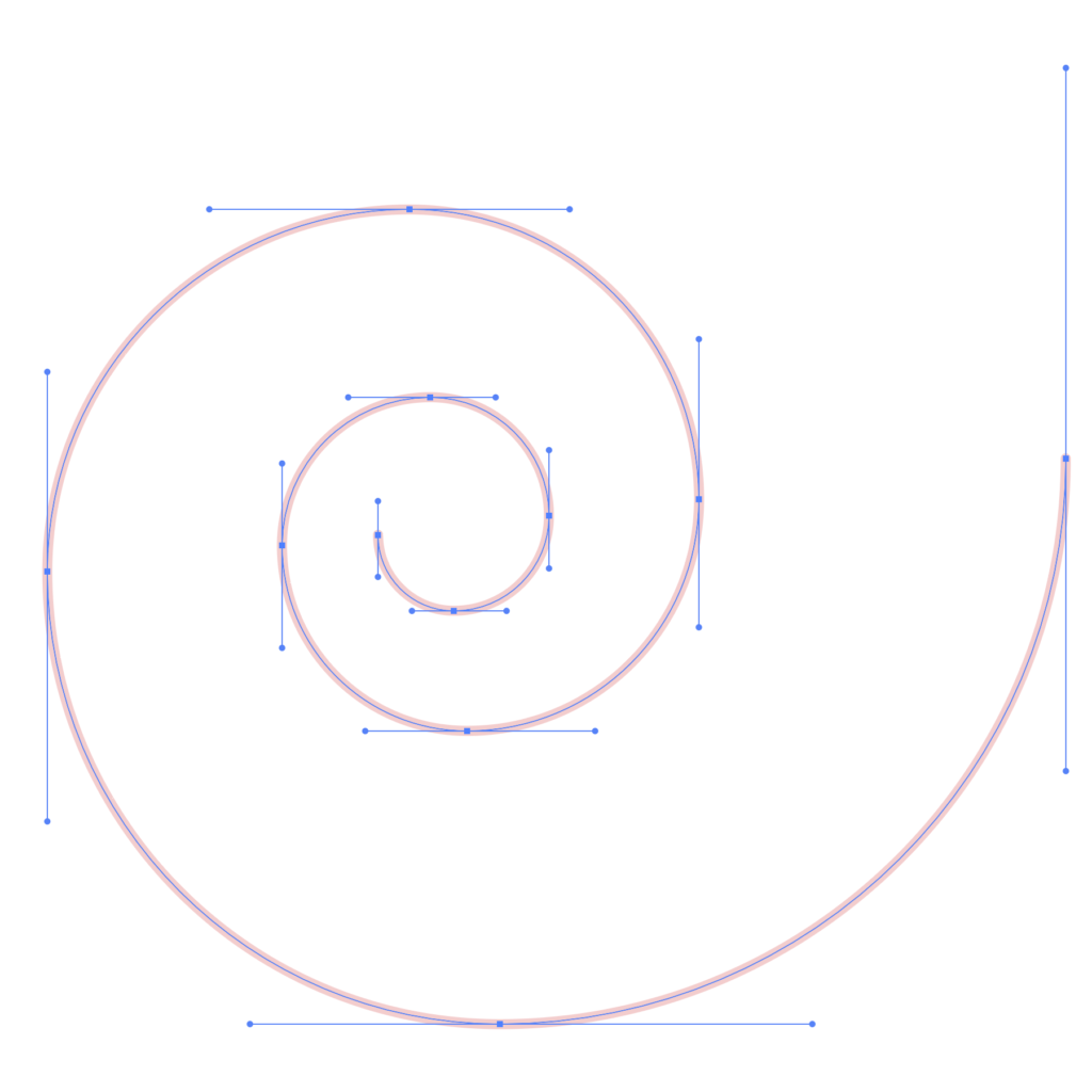
Think about a 2D curve analogy. In the spiral seen here, as the curve gets tighter, we see more frequent anchor points and Bezier handles. As we travel to the larger end of the curve, anchors are less frequent. This principle of economy is also what drives good subdivision practice, and Subdiv models in Maya achieve a similar economy in 3D. However, because Subdivs are exclusive to Maya as a modeling type, we must convert them to polygons or NURBS to make something with them. That said, they are excellent for achieving the smoothing most models require, without the overhead of unnecessary faces we get with smoothing alone.
Smoothing strategies
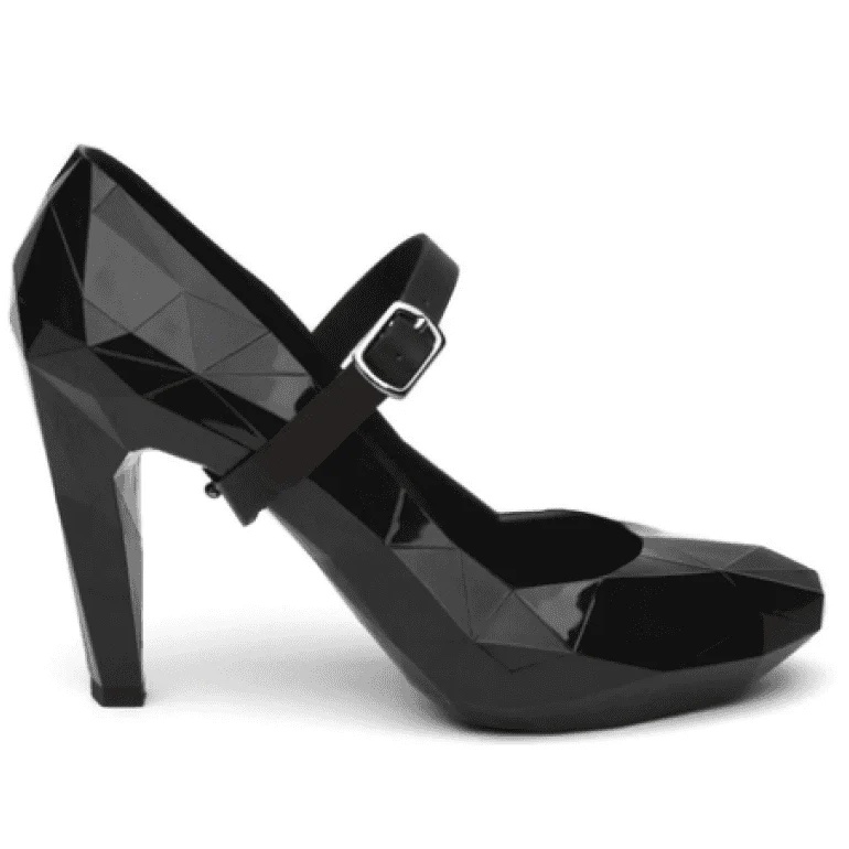
This Lo-Res shoe is a metatextual commentary on its origins as a model for fabrication. The designer, Rem Koolhaas, exaggerates and expresses in hard edges the low-resolution polygonal model used to manufacture the shoe. In most instances, however, the goal is for such a model to be as smooth as possible.
Let’s look at a common example of subdivisions for smoothing: a hand. In the illustration, at the far left, we see a basic hand model in progress for which we have developed fingernails and knuckles. It’s very blocky but exhibits good edge flow, and it contains about 600 polygons, most of which are quads.
In the top row, we see a basic strategy for smoothing. At the top center, we treat the model with a smooth mesh preview (key 3), but this doesn’t subdivide it yet. When we apply a Modify > Convert > Smooth Mesh Preview to Polygons, seen at the top right, we arrive at a smoother model with 9300 polygons. This creates additional polygons where we want them at the fingernails and knuckles, but we also find extra geometry where we don’t, like the back of the hand.
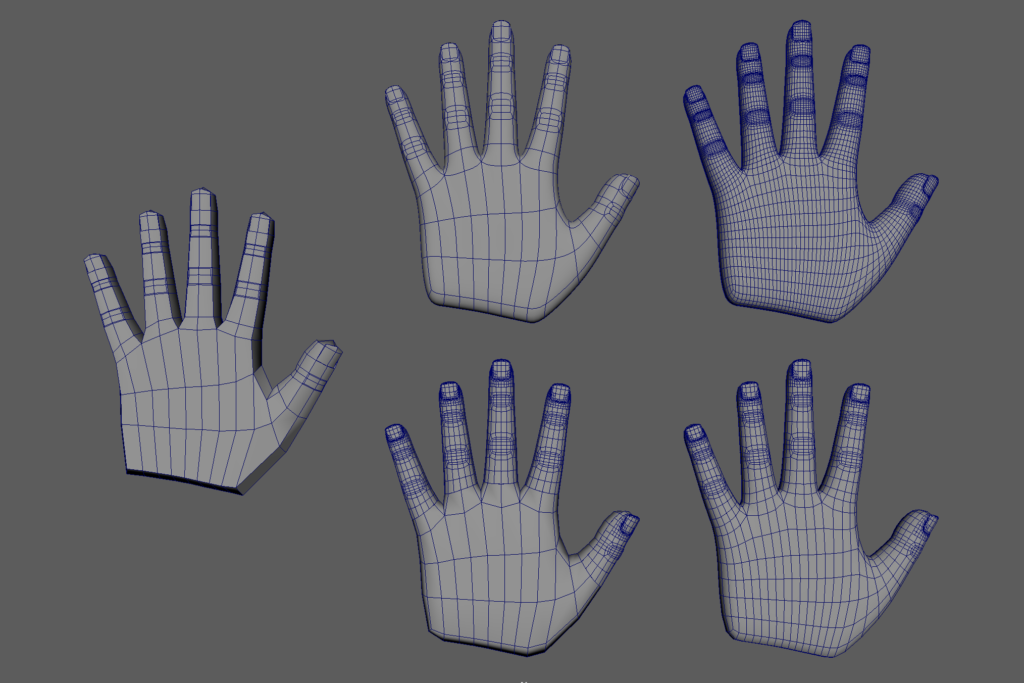
In the bottom row, we apply Modify > Convert > Polygons to Subdivs, and the difference is apparent. This creates much more geometry at the detail from the get-go. Then, when we apply Modify > Convert > Subdivs to Polygons, we see a polygon model with only 3100 polygons, a third of what we get with keyboard 3 smoothing.
Micro-beveling
With the quad ball above, we see what happens when we smooth preview a cube with no subdivisions. But if we want to keep its “cubeness” intact, we can introduce a Micro-bevel.
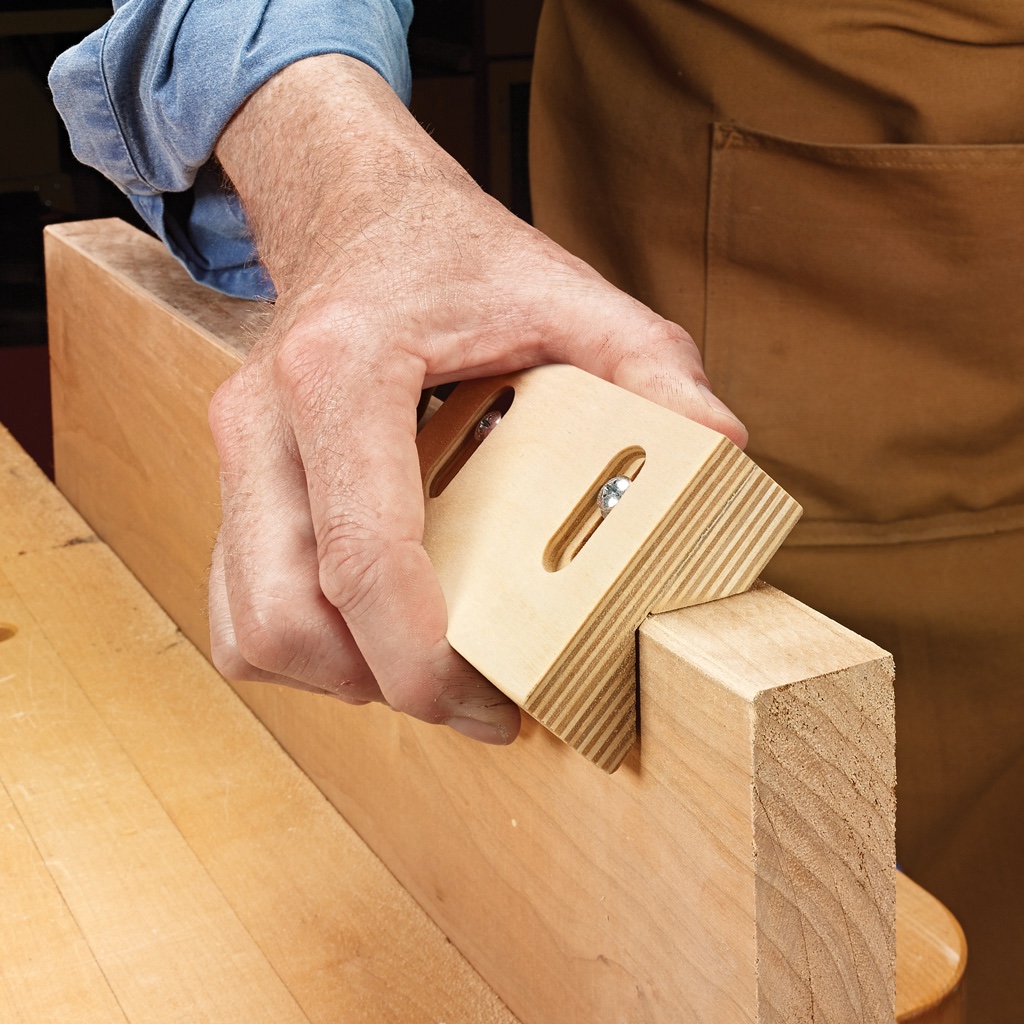
In woodworking, to avoid sharp splinter-filled edges, we knock them down by sanding. These are variously called bevels, fillets, or chamfers, and 3D programs use these terms to describe tools to knock down the corners of models. A fillet is rounded, while bevels and chamfers are variations on angles. In a polygon model, the knockdown corner will be chamfer-like, but a smooth mesh preview appears to be a rounded fillet. We use micro-bevel as a generic term to refer to these edge treatments.
The micro-bevel solves two problems. The first is that a hard-edge model is a little too perfect, with results that feel artificial, especially if the goal is photo-realistic rendering. Micro-beveling provides a rendered sense of authentic materiality.
The second is the level of control we have over the knockdown. In our sample, we see a polygon primitive cube and its smooth mesh preview at left. At center, we’ve applied 3 subdivisions, so when we apply smoothing, we get a soft corner, but it’s rather large. For a smaller knockdown, we’d need to apply too many subdivisions. So instead we use the Bevel tool with a small fractional value on the cube at right. When softened, we get a micro-bevel using the same number of faces as the softened center cube!
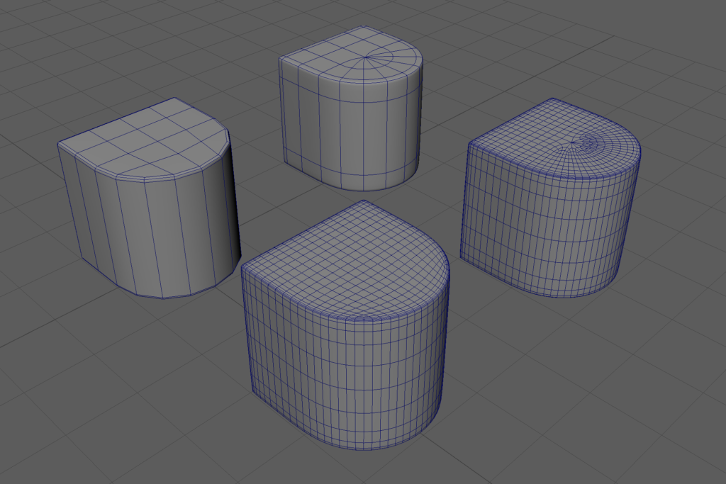
How about micro-bevels on non-cubic shapes like the cube-cylinder combination illustrated? On the solution at left, we develop an edge flow exclusively made of quads. In the one on the right, we have a group of polar rectangles creating a pinch in the top plane.
Converting geometries: a workflow case study
When modeling, don’t fall into the trap of thinking “I’ll only use polygons because they’re easier” or “I’m designing so I can only use NURBS.” If we’re working with Maya we can find it useful to migrate the work from one modeling environment to another using the Convert functions. We find a great example of this flexibility in the workflow used to model a wine glass.
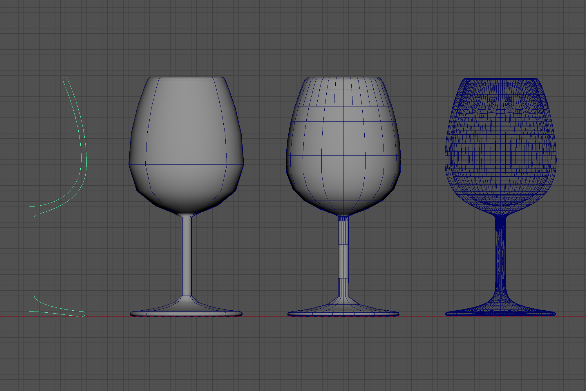
We start the wine glass with a simple NURBS curve tracing the outline of one-half of the glass, then apply a NURBS Revolve function to it. From that object, we use Modify > Convert > NURBS to Polygons to arrive at a polygon model, to which we apply smoothing. Lastly, we use Modify > Convert > Smooth Mesh Preview to Polygons to get to the final super-smoothed form.
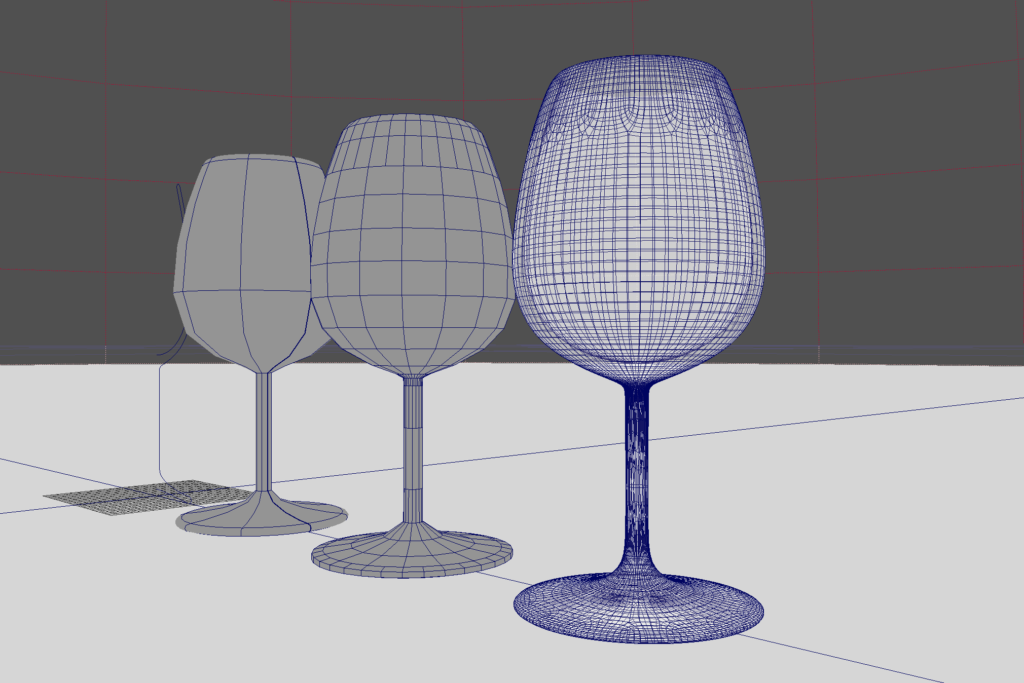
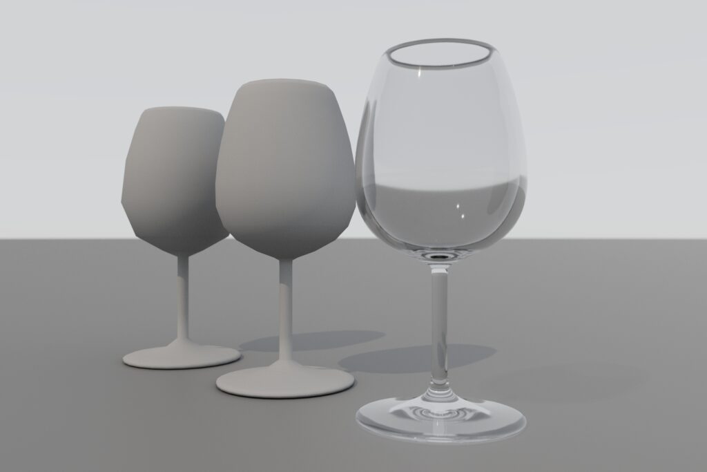
When we apply a glass material to the final model, we get excellent refraction and reflection results! It would take forever to beat a polygon primitive cylinder into the wine glass shape with the requisite thin wall. With this workflow, the time-consuming part is the creation of the initial NURBS curve, but this only takes minutes, not hours. From there, the revolve and smoothing conversion functions are comparatively quick.